Usage
Our tool uses published methods to extract summary sleep and activity statistics from accelerometer data.
Basic usage
To extract a summary of movement metrics from raw Axivity files (.cwa):
$ accProcess data/sample.cwa.gz
<summary output written to data/sample-summary.json>
<time-series output written to data/sample-timeSeries.csv.gz>
See CLI and API reference for more details.
This will output a number of files, described in the table below. The files Epoch.csv and NonWearBouts.csv are optional.
File |
Description |
|---|---|
Summary.json |
Summary statistics for the entire input file, such as data quality, acceleration and non-wear time grouped hour of day, and histograms of acceleration levels. |
TimeSeries.csv |
Acceleration time-series and predicted activities (if enabled). |
Epoch.csv |
Acceleration data grouped in epochs (default: 30sec). Detailed information about XYZ acceleration, standard deviation, temperature, and data errors can be found in this file. |
NonWearBouts.csv |
Start and end times for any non-wear bouts, and the detected (presumably low) acceleration levels for each bout. |
To visualise the output time-series:
$ accPlot data/sample-timeSeries.csv.gz
<output plot written to data/sample-timeSeries-plot.png>
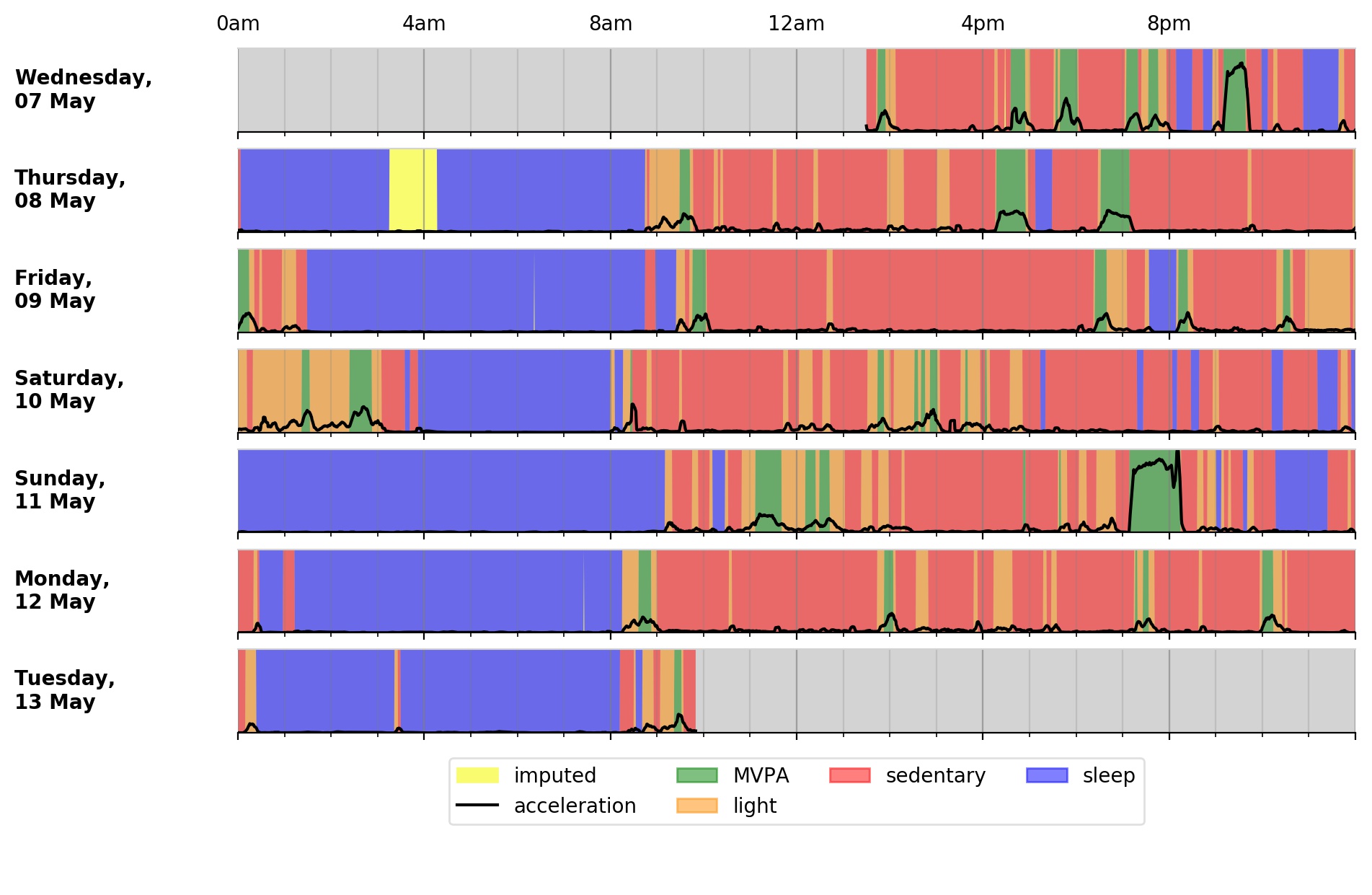
Output plot of overall activity and class predictions for each 30sec time window
Processing a CSV file
$ accProcess data/sample.csv.gz
The CSV file must have at least four columns: a time column and three other columns corresponding to the tri-axial acceleration values. A template can be downloaded as follows:
$ wget "http://gas.ndph.ox.ac.uk/aidend/accModels/sample-small.csv.gz"
$ mv sample-small.csv.gz data/
$ gunzip data/sample.csv.gz
$ head -3 data/sample.csv
time,x,y,z
2014-05-07 13:29:50.439+0100 [Europe/London],-0.514,0.07,1.671
2014-05-07 13:29:50.449+0100 [Europe/London],-0.089,-0.805,-0.59
If your CSV is in a different format, there are options to flexibly parse these. Consider the below file with a different time format and the x/y/z columns in different order:
$ head data/awkwardfile.csv
time,temperature,z,y,x
2014-05-07 13:29:50.439,20,0.07,1.671,-0.514
2014-05-07 13:29:50.449,20,-0.805,-0.59,-0.089
The above file can be processed as follows:
$ accProcess data/awkwardFile.csv \
--csvTimeFormat 'yyyy-MM-dd HH:mm:ss.SSS' --csvTimeXYZTempColsIndex 0,4,2,3
If your CSV also has a temperature column, it is possible to include it:
$ accProcess data/awkwardFile.csv \
--csvTimeFormat 'yyyy-MM-dd HH:mm:ss.SSS' --csvTimeXYZTempColsIndex 0,4,2,3,1
Processing multiple files
Suppose you want to process hundreds of accelerometer files:
studyName/
    subject001.cwa
    subject002.cwa
    subject003.cwa
    ...
We provide utility command line tools to facilitate generating the list of commands to process each file:
$ accWriteCmds myStudy/ -d myStudyResults/ -f list-of-commands.txt
<list of processing commands written to "list-of-commands.txt">
A list-of-commands.txt text file will be created listing the processing commands
for each file under myStudy/.
By default, the tool will search for all Axivity (.cwa) files.
To process other file types, use the --accExt flag. For example:
# Process Actigraph (.gt3x) files
$ accWriteCmds myStudy/ -d myStudyResults/ -f list-of-commands.txt --accExt gt3x

# Process GENEActiv (.bin) files
$ accWriteCmds myStudy/ -d myStudyResults/ -f list-of-commands.txt --accExt bin
If you need to pass extra arguments to the processing commands, you can use the
-x flag, then pass the arguments within quotation marks. For example,
below we pass the arguments --mgCutPointMVPA 90 and
--mgCutPointVPA 435 to customise the cutpoints for MVPA and VPA:
$ accWriteCmds myStudy/ -d myStudyResults/ -f list-of-commands.txt -x '--mgCutPointMVPA 90 --mgCutPointVPA 435'
<list of processing commands written to "list-of-commands.txt">
Once the list-of-commands.txt file has been created, you can kick-start the list of processes:
Note
More advanced users will probably want to parallelise the below script.
$ bash list-of-commands.txt
Following the example, the results will be stored in myStudyResults/ as follows:
myStudyResults/
    subject001/
        subject001-timeSeries.csv
        subject001-summary.json
        ...
    subject002/
        subject002-timeSeries.csv
        subject002-summary.json
        ...
    ...
Finally, you can collate all the summary JSON files into a single large csv for subsequent analyses:
$ accCollateSummary myStudyResults/ -o summary.csv
<summary CSV for all participants written to "summary.csv">
Classifying different activity types
Different activity classification models can be specified to identify different activity types. For example, to use activity types from the Willetts 2018 Scientific Reports paper:
$ accProcess data/sample.cwa.gz --activityModel willetts
To visualise the time series and new activity classification output:
$ accPlot data/sample-timeSeries.csv.gz
<output plot written to data/sample-timeSeries-plot.png>
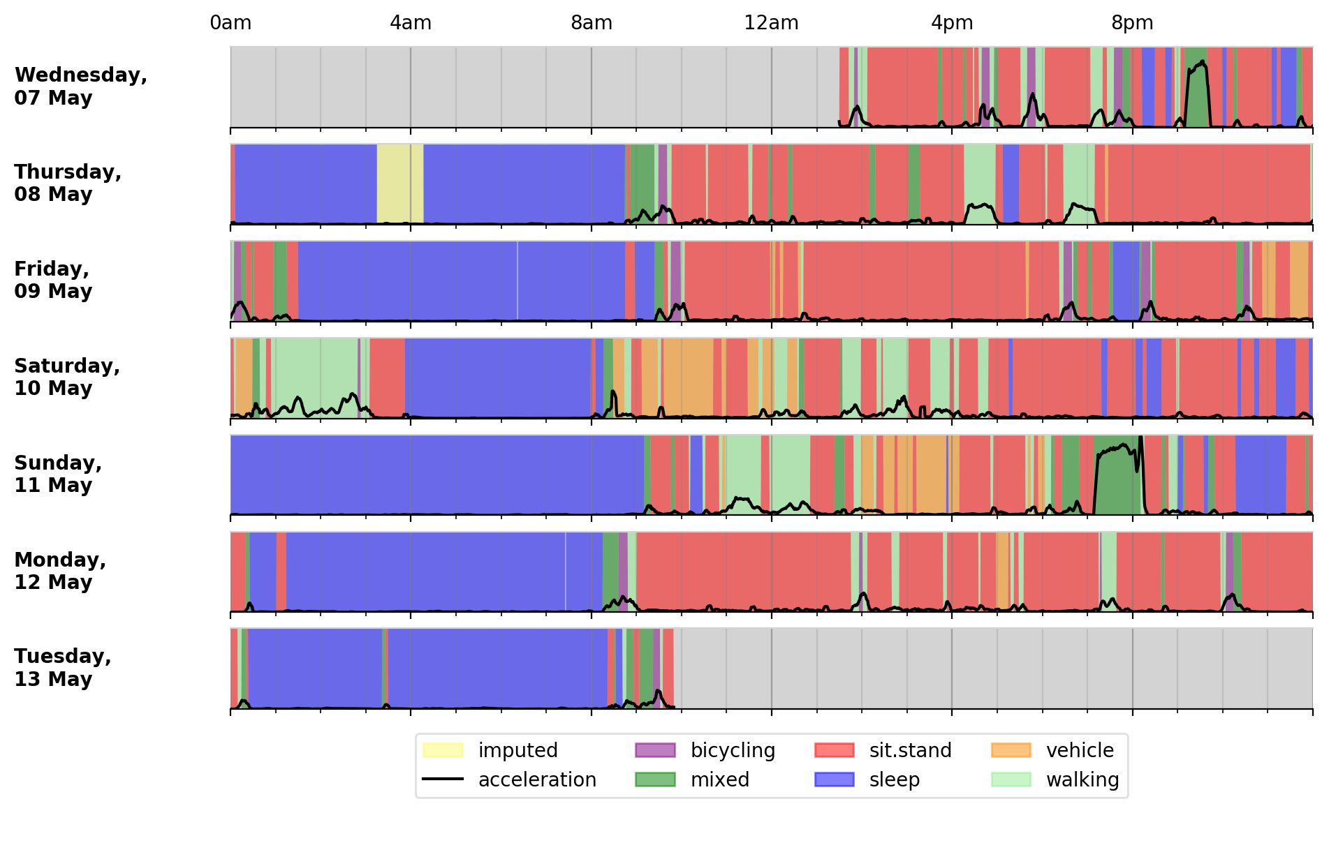
Output plot of class predictions using Willetts 2018 classification model. Note different set of activity classes.
Training a bespoke model
It is also possible to train a bespoke activity classification model. This requires a labelled dataset (.csv file) and a list of features (.txt file) to include from the epoch file.
First we need to evaluate how well the model works on unseen data. We therefore train a model on a ‘training set’ of participants, and then test how well that model works on a ‘test set’ of participant. The command below allows us to achieve this by specifying the test participant IDs (all other IDs will automatically go to the training set). This will output <participant, time, actual, predicted> predictions for each instance of data in the test set to a CSV file to help assess the model:
import accelerometer
from accelerometer.classification import trainClassificationModel
trainClassificationModel( \
    "labelled-acc-epochs.csv", \
    featuresTxt="features.txt", \
    testParticipants="4,5", \
    outputPredict="test-predictions.csv", \
    rfTrees=1000, rfThreads=1)
# <Test predictions written to:  test-predictions.csv>
A number of metrics can then be calculated from the test predictions csv file:
import pandas as pd
from accelerometer import classification

# load data
data = pd.read_csv("test-predictions.csv")

# print summary to HTML file
htmlFile = "classificationReport.html"
yTrueCol = 'label'
yPredCol = 'predicted'
participantCol = 'participant'
classification.perParticipantSummaryHTML(data, yTrueCol, yPredCol,
    participantCol, htmlFile)
After evaluating the performance of our model on unseen data, we then re-train a final model that includes all possible data. We therefore specify the outputModel parameter, and also set testParticipants to ‘None’ so as to maximise the amount of training data for the final model. This results in an output .tar model:
from accelerometer.classification import trainClassificationModel
trainClassificationModel( \
    "labelled-acc-epochs.csv", \
    featuresTxt="features.txt", \
    rfTrees=1000, rfThreads=1, \
    testParticipants=None, \
    outputModel="custom-model.tar")
# <Model saved to custom-model.tar>
This new model can be deployed as follows:
$ accProcess data/sample.cwa.gz --activityModel custom-model.tar
See CLI and API reference for more details.
Leave one out classification
To rigorously test a model with training data from <200 participants, leave one participant out evaluation can be helpful. Building on the above examples of training a bespoke model, we use python to create a list of commands to test the performance of a model trained on unseen data for each participant:
import pandas as pd
from acceleration.classification import trainClassificationModel

trainingFile = "labelled-acc-epochs.csv"
d = pd.read_csv(trainingFile, usecols=['participant'])
pts = sorted(d['participant'].unique())

w = open('training-cmds.txt','w')
for p in pts:
    cmd = "import accelerometer;"
    cmd += "trainClassificationModel("
    cmd += "'" + trainingFile + "', "
    cmd += "featuresTxt='features.txt',"
    cmd += "testParticipants='" + str(p) + "',"
    cmd += "labelCol='label',"
    cmd += "outputPredict='testPredict-" + str(p) + ".csv',"
    cmd += "rfTrees=100, rfThreads=1)"
    w.write('python3 -c $"' + cmd + '"\n')
w.close()
# <list of processing commands written to "training-cmds.txt">
These commands can be executed as follows:
$ bash training-cmds.txt
After processing the train/test commands, the resulting predictions for each test participant can be collated as follows:
$ head -1 testPredict-1.csv > header.csv
$ awk 'FNR > 1' testPredict-*.csv > tmp.csv
$ cat header.csv tmp.csv > test-predictions.csv
$ rm header.csv
$ rm tmp.csv
More examples
To list all available processing options and their defaults:
$ accProcess -h
If a path has spaces, enclose it within quotes:
$ accProcess '/path/to/my file.cwa'
Change epoch length to 60 seconds:
$ accProcess data/sample.cwa.gz --epochPeriod 60
Manually set calibration coefficients:
$ accProcess data/sample.cwa.gz
    --skipCalibration True \
    --calOffset -0.2 -0.4 1.5 \
    --calSlope 0.7 0.8 0.7 \
    --calTemp 0.2 0.2 0.2
Convert a CWA file to CSV (resampled and calibrated):
$ accProcess data/sample.cwa.gz --rawOutput True
Plot just the first few days of a time-series file (e.g. n=3):
$ accPlot data/sample-timeSeries.csv.gz --showFirstNDays 3
Quality control
Check this notebook for guidance on how to perform quality control on studies involving large number of accelerometers.
Tool versions
Data processing methods are under continual development. We periodically retrain the classifiers to reflect developments in data processing or the training data. This means data processed with different versions of the tool may not be directly comparable. In particular, to compare returned variables in UK Biobank and external data, we recommend:
Either, reprocessing UK Biobank data alongside external data;
Or, using a version of the models and software to process external data which matches that used to process the returned UK Biobank data (to be achieved from November 2021 onwards through versioning of the package and associating each set of processed data with a particular version).